| Issue |
Res. Des. Nucl. Eng.
Volume 2, 2026
|
|
|---|---|---|
| Article Number | 2025008 | |
| Number of page(s) | 9 | |
| DOI | https://doi.org/10.1051/rdne/2025008 | |
| Published online | 17 February 2026 | |
Research Article
Trip transient analysis on the main feedwater pump of HPR1000
1
Laiyang Nuclear Power Co., Ltd, Yantai 265200, China
2
Hebei Branch, China Nuclear Power Engineering Co., Ltd., Shijiazhuang 050021, China
3
Key Laboratory of Low-Grade Energy Utilization Technologies and Systems, Chongqing University, Chongqing 400044, China
4
School of Energy and Power Engineering, Chongqing University, Chongqing 400044, China
5
School of Business, Society and Engineering, Mälardalen University, 721 23 Västerås, Sweden
* e-mail: This email address is being protected from spambots. You need JavaScript enabled to view it.
Received:
30
June
2025
Accepted:
24
October
2025
Abstract
In PWR, the main feedwater pump is one of the main equipment in the secondary side which has an important impact on the safe and stable operation of the entire power plant, and then directly affecting the output and availability of the unit. Based on the system manual and equipment data of a HPR1000 nuclear power unit, a mathematical model including the deaerator system and main feedwater pump system was established on the APROS platform. Through transient simulation and calculations of the main feedwater pump trip, it was shown that the load reduced to 50% FP quickly when backup pump for the tripping main feedwater pump did not start, and which can avoid reactor shutdown caused by low steam generator water level, whereas the three initial conditions of unit are 90% FP, 80% FP, and 70% FP. The comparison of debugging test data and the simulation data of a feedwater pump tripping under an initial load of 70% FP shows that the data is in good agreement, and the error between the experimental data and the simulation data for initial and final values of the deaerator pressure is within 1.5%. The flowrate error between the debugging test data and the simulation data of the tripping pump is about 8.1%, and the maximum flowrate error between the debugging test data and the simulation data for the normal operation pump overspeed operation is about 2‰, and the flowrate error between the debugging test data and the simulation data after stabilizing at 50% FP is about 10.1%. The mathematical model established in this paper can effectively predict the changes in deaerator pressure and liquid level, feedwater pump flowrate under transient conditions of a single feedwater pump failure and trips. The modeling method for the main feedwater pump, deaerator, and other systems and equipment used in this paper, as well as the boundary condition assumptions for calculating the operating conditions, can provide reference for the design of the subsequent HPR1000 nuclear power unit.
Key words: HPR1000 / Main feedwater pump / Pump trip / Transient analysis / Debugging test
© J. Yang et al. 2026. Published by EDP Sciences.
 This is an Open Access article distributed under the terms of the Creative Commons Attribution License (https://creativecommons.org/licenses/by/4.0), which permits unrestricted use, distribution, and reproduction in any medium, provided the original work is properly cited.
Abbreviation List
APROS: Advanced Process Simulation Software
CFX: Ansys CFX
CENTS: CENTS Program
DCS: Distributed Control System
DEC: Design Extension Condition
FP: Full Power
HPR1000: HPR1000 (Hua Long One)
Matlab/Simulink: Matlab/Simulink
MSGTR: Main Steam Line Break with Gamma Ray Release
MW: Megawatt
NPSH: Net Positive Suction Head
PI: Proportional-Integral
PWR: Pressurized Water Reactor
SBLOCA-LOSI: Small Break Loss of Coolant Accident with Loss of Shutdown Cooling Injection
SBO: Station Blackout
SG: Steam Generator
1 Introduction
In PWR power plants, the main feedwater pump is one of the main important equipment in the secondary side. Although operating conditions of the main feedwater pump does not affect nuclear safety directly, the equipment status of main feedwater pump has an important impact on the output and availability of the unit. The main feedwater pump transport saturated water and was operated in the conditions of high flowrate and high head. Due to the complex working environment, if the standby pump failed to auto-start when one of the running main feedwater pumps tripped, the reactor needs to be shut down immediately. The above operational events have been reported in several domestic PWR power units.
In the field of modeling and simulation for feedwater pumps in traditional thermal power units, relevant scholars have conducted targeted research focusing on different unit types and technical pain points: Based on Ansys CFX software, G. Pan et al. [1] employed the standard k-ε turbulence model to perform 3D flow field numerical calculations for feedwater pumps in ultra-supercritical 1000 MW units. They obtained the velocity and pressure distributions of key components such as impellers and guide vanes. The relative errors between the predicted head values and experimental values ranged from 1.8% to 7.8%, and the relative errors in efficiency were between 3.8% and 6.3%, which verified the effectiveness of the full-flow channel model. H. Li et al. [2] established a mathematical model and a Matlab simulation model for the feedwater pump turbine, and analyzed its stability under step speed disturbances. The results showed that the speed reached a steady state within 10–25 s, which could meet the boiler feedwater regulation requirements. W. Li et al. [3] constructed load-specific models for the feedwater system of a 600 MW subcritical unit using Matlab/Simulink. They addressed the coupling issue between drum water level and bypass control valve differential pressure under low loads, as well as the false water level interference under high loads. After optimization, the low-load water level overshoot, decay rate, and high-load variable-condition water level stability all reached excellent indicators. For 142 MW heating units, L. Fu [4] added a control loop for the steam-driven pump to regulate the drum water level of a single boiler and an over/under-pressure protection loop for the feedwater header through DCS software configuration. This realized the reasonable adaptation of the “one boiler with one turbine” and “two boilers with one turbine” operation modes, and avoided the risk of boiler shutdown caused by control valve jamming. D. Li et al. [5] constructed a dynamic model of feedwater pumps considering the influence of cavitation, quantified the relationship between the required net positive suction head (NPSH) and cavitation degree, and used a first-order inertial link to characterize the pump start-stop process, providing an effective method for simulating feedwater pump cavitation faults. Regarding the establishment of feedwater pump models for nuclear power units, X. Cheng et al. [6] used the CENTS program to conduct simulation analysis of the main feedwater pump tripping process in AP1000 units, and presented the variation laws of data such as nuclear power, turbine power, primary loop coolant temperature, and steam generator (SG) liquid level. B. Zeng et al. [7] analyzed the tripping transient of the main feedwater pump in a certain M310 nuclear power unit and optimized the design of the pump warm-up system. Y. Hu [8] studied the rated flow rate, head, and related margin selection of main feedwater pumps in pressurized water reactor (PWR) nuclear power plants, and put forward suggestions on margin values. L. Zhao [9] used APROS to model and simulate the secondary loop of the Hongyanhe nuclear power unit, and verified the simulation of unit operating states with deviations from design conditions, such as changes in circulating water parameters, condenser tube blockage, and increased extraction pressure loss of heaters. The above simulation results showed high consistency with on-site data, verifying the accuracy of the model. When a main feedwater pump trips, if the backup pump fails to start, the main feedwater flow rate in the secondary loop and the turbine power will decrease. Consequently, parameters such as the working fluid flow rate and enthalpy change rapidly, which exerts a significant impact on the stable operation of the steam generator (SG) and the primary loop. This impact is intuitively reflected in the changes in SG pressure and water level.
Regarding the research on the dynamic characteristics of deaerators under transient operating conditions, there are two main commonly used methods worldwide. One is to establish a dynamic model of the deaerator using simulation software and identify the factors affecting deaerator pressure and liquid level through operating condition simulation; the other is to obtain predicted operating data of the deaerator’s dynamic characteristics under off-design conditions by analyzing experimental data of transient operating conditions. Given that the interior of the deaerator is in a saturated vapor-liquid two-phase state, it is impossible to fully cover its characteristics under variable operating conditions through experimental methods. Therefore, the most economical and convenient approach is to acquire the variation laws of the deaerator’s dynamic characteristic data under various off-design conditions via software modeling and transient operating condition simulation [10]. Currently, the widely recognized mathematical model globally is mainly the Iving model, and some large-scale commercial software also has built-in general models for other deaerators. However, the calculation accuracy and response speed of the aforementioned models are hardly able to meet the special operating requirements of deaerators in nuclear power units [11]. Yukihiro et al. [12] proposed a model algorithm based on neural networks and applied it to the simulation analysis of the deaerator liquid level control system, achieving favorable results.
For the predictive analysis of the operational characteristics of main feedwater pumps and deaerators, some studies adopt the large-scale general transient analysis software APROS for modeling, while others use the CENTS program and the large-scale control analysis software Matlab/Simulink to conduct simulation analysis of the main feedwater control system. Regardless of the program employed, the key lies in determining appropriate boundary conditions and accurate operation sequences.
The research object of this paper, HPR1000 (China’s independent third-generation nuclear power technology), is independently developed and researched by China, which holds complete independent intellectual property rights for it [13]. The tripping of the main feedwater pump is one of the important commissioning tests before a unit enters commercial operation. In the HPR1000 series units, 3 × 50% electric feedwater pumps are configured; during normal unit operation, two pumps are in service and one is on standby. Taking the main feedwater pump set of a certain HPR1000 nuclear power unit as the research subject, this paper uses APROS software to establish a simulation model of systems and equipment including deaerators and main feedwater pumps. It conducts simulation analysis on the variation trends of pressure and liquid level in the deaerator, as well as the flow variation laws of normal pumps and faulty pumps, under the transient condition where one pump trips and the backup pump fails to start. Furthermore, comparative verification is carried out between the simulation analysis data and commissioning test data, providing reference data and basis documents for the design, commissioning, and operation of subsequent similar units.
2 Numerical calculation models and simulation algorithms
The purpose of mathematical modeling is to simulate the dynamic behavior of the secondary circuit system in nuclear power units based on HPR1000. The main thermal and hydraulic components of the secondary circuit include steam and water supply circuit pipes, turbine high-pressure cylinder, intermediate pressure cylinder, low-pressure cylinder, moisture steam separator and steam reheating heater, condenser, deaerator, feedwater pump, regulating valve, etc. (as shown in Fig. 1). By incorporating a PI control model, the study of the variable operating conditions characteristics of the model has been achieved. The main mathematical models of the equipment are detailed in the following text.
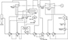 |
Figure 1 Thermal system diagram of the secondary loop. |
2.1 Deaerator model
This study adopts the Lumped Parameter Model to construct the mathematical model of the deaerator. Its core definition is as follows: it ignores the distribution differences of spatial parameters (such as temperature, pressure, and concentration) inside the equipment, regards the deaerator as a single centralized control volume, and describes its dynamic characteristics using overall average parameters (such as average pressure, average liquid level, and average temperature). This model assumes that the parameters of the working fluid inside the deaerator only change with time rather than spatial position. It is suitable for analyzing the overall dynamic response of the system (e.g., the variation trends of pressure and liquid level under transient conditions) rather than local microscale characteristics, which meets the research needs of this study regarding the main feedwater pump tripping transient.
The simulation calculations in this study are based on the APROS (Advanced Process Simulation Software) platform, which is developed by the VTT Technical Research Centre of Finland. As a large-scale general-purpose transient simulation software for thermal systems, it is equipped with a high-precision equipment model library, flexible boundary condition configuration functions, and an efficient numerical solver. It can accurately simulate the dynamic characteristics of complex thermal systems such as nuclear power plants and thermal power plants, providing a reliable environment for model construction and transient calculations in this study.
The boundary conditions assumed in the model of the deaerator are:
-
The deaerator model is a lumped parameter model, and water is assumed as an incompressible fluid;
-
Convective heat transfer is carried out between heated steam, drain water, and condensate water, without considering the influence of non-condensable gases on condensation rate. The vapor and liquid inside the deaerator are in phase equilibrium;
-
Consider the heat storage capacity of the metal and heat exchange between the body of the deaerator cylinder and water, with each point of the deaerator cylinder is at the same temperature, without considering heat dissipation to the environment.
The mathematical models of deaerator mainly include mass conservation equation and energy conservation equation, as follows:
The conservation equation of mass on the steam side [14]: (1)
(1)
Conservation equation of mass on the water side: (2)
(2)
The energy conservation equation in the deaerator: (3)
(3)
-
 ,
,  – Density of working fluid on the steam or water side, kg/m3;
 -
 ,
,  – Volume of working fluid on the steam or water side, m3;
 -
 ,
,  – Heating steam inflow into the deaerator, heating steam outflow from the deaerator, steam condensation rate, condensate water inflow into the deaerator, water outflow from the deaerator, amount of saturated water and saturated steam stored in the deaerator, kg/s;
 -
 ,
,  ,
,  ,
,  ,
,  ,
,  – saturated water enthalpy, saturated vapor enthalpy, inlet water enthalpy of deaerator, outlet water enthalpy of deaerator, deaerator, inlet steam enthalpy of running exhaust steam enthalpy of deaerator R, kJ/kg;
 -
 – Total volume of deaerator, m3;
 -
 – Steam saturation pressure, Pa.
Water level equation:
Water level: (4)
(4)
Cross section area of water: (5)
(5)
-
 – Water level height inside the deaerator, mm (the common unit of water level height in the deaerator is mm);
 -
A – cross-sectional area of water inside the deaerator, m2;
-
R – radius of deaerator water tank, m;
-
θ – Angular radians as shown in Figure 2.
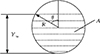 |
Figure 2 Schematic diagram of deaerator water level calculation. |
In the process of rapid load reduction, a six-equation model based on one-dimensional conservation equation is adopted for simulation and calculation, considering the phase change and heat transfer process. The model equation is as follows: (6)
(6)
 (7)
(7)
 (8)
(8)
 refers to the void fraction of the working fluid. The subscript k in the equation represents the working fluid state (vapor-v/water-w), i represents the steam-water interface, and m represents the metal cylinder wall. Γ Represents the mass flow rate of steam-water conversion (positive for evaporation process and negative for condensation process), F represents frictional force (including valve and frictional force along the tube), Q is the heat transfer at the interface,
  is the pressure head loss of the pump, and h represents the total enthalpy including kinetic energy [15].
The interfacial heat transfer Q in equation (8) is calculated according to the following equations respectively in the steam and water phases,
Steam phase: (9)
(9)
Water phase: (10)
(10)
In equations (9) and (10), k is the heat transfer coefficient, and  is the saturation enthalpy.
The mass flow rate in the phase change zone is calculated using the two-phase heat transfer equation: (11)
(11)
2.2 Main feedwater pump group model
The electric driven main feedwater pump group consists of a centrifugal pre pump and a pressure stage pump, an electric motor, and a hydraulic coupling. Based on the characteristic curves and similarity relationships provided by the supplier for the pre pump and pressure stage pump, the simulation operation of the pump under off-design working conditions is extrapolated. When establishing a pump group model, consider the pump is in the steady-state operation, without cavitation, backflow, and insulation, and consider the rotational inertia of the pump, motor, and hydraulic coupling, but do not consider the loss of mechanical sealing medium.
The head of a pump is expressed as the relationship between pressure head, velocity head, and position head, as follows [16]: (12)
(12)
In equation (12):
-
 ,
, – static pressure strength of liquid at pump outlet and inlet, Pa;
 -
 ,
, – The velocity of liquid at the pump outlet and inlet, m/s;
 -
 ,
, – The elevation of the pump at the outlet and inlet relative to the reference plane, m;
 -
ρ – The fluid density transported by the pump, kg/m3.
The power that a pump can transmit to the fluid per unit time is expressed as effective power, expressed in  , as follows:
 (13)
(13)
In equation (13):
-
ρ – Density of liquid, kg/m3;
-
 – Gravitational acceleration, m/s2;
 -
 – Volume flow rate of fluid passing through the pump, m3/s;
 -
H-pump head, mH2O.
The speed of pump can be calculated by the following equation: (14)
(14)
In equation (14):
-
 , motor inertia, kg/m2;
 -
 , pump inertia, kg/m2;
 -
 , frequency, Hz;
 -
 , torque, N∙m.
2.3 Numerical algorithm
The mathematical model for the entire nuclear power unit is of large scale, covering numerous systems and equipment. The general deaerator equipment model built in APROS is presented in the form of ordinary differential equations (ODEs). For the solution of such ODEs, based on defined initial and boundary conditions, the problem of solving real-variable equations is converted into an initial-value problem of ODEs.
There are various numerical solution methods for ODE systems. Among them, the Gear algorithm has the advantages of high accuracy and strong stability when solving stiff differential equations, which can effectively adapt to the rapid parameter changes during the transient process of nuclear power units. Therefore, this study selects the Gear algorithm as the core numerical calculation method for transient simulation to ensure the accuracy of simulation results for key parameters such as deaerator pressure and feedwater pump flow rate.
3 Transient calculation results and verification
3.1 Initial operating conditions
This paper calculated the transient process of the unit from three stable initial conditions of 90% FP, 80% FP, and 70% FP. After a single feedwater pump trips, the unit quickly reduces load to 50% FP, and the evolution process of deaerator pressure and liquid level, flow rate of normal operation pump and fault pump were calculated.
Transient process: At t = 10 s, one main feedwater pump tripped and the backup pump failed to start. Subsequently, the normal main feedwater pump ran at the maximum speed for 15 s. The output load was quickly reduced to 50% FP for operation.
3.2 Changes in pressure and liquid level of deaerator
Figures 3 and 4 show the changes in deaerator pressure and liquid level over time under three initial operating conditions: 90% FP, 80% FP, and 70% FP, after a feedwater pump trips and the backup pump failed to start. To verify the accuracy of simulation data, a comparison was made between simulation data and debugging test data. In the debugging test data of a certain HPR1000 unit, the test data of one main feedwater pump tripping and the standby pump not starting when the unit is operating at 70% FP initial load are provided.
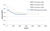 |
Figure 3 Pressure variation of deaerator over time. |
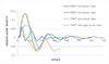 |
Figure 4 Changes in deaerator water level over time. |
According to the transient simulation data in Figure 3, it can be seen that after a running feedwater pump trips, due to the rapid decrease in output load, the extraction pressure of the deaerator decreases rapidly, and the saturated water inside the deaerator flashes. The internal pressure of the deaerator increases at first and then decreases slowly. The internal pressure change trend of the deaerator is consistent under three initial operating conditions: 90% FP, 80% FP, and 70% FP, there is a pattern of first increasing and then decreasing in all cases. According to the pattern of the pressure curve in the deaerator, the lower the initial load, the smaller the increase amplitude in deaerator pressure during the transient process. Finally, the deaerator pressure stabilizes at 0.52 MPa.
Comparing the transient simulation data under the initial load of 70% FP with the unit debugging test data, it was found that the initial pressure inside the deaerator was 0.7 MPa and 0.71 MPa, respectively, and the stable pressure of the unit was both 0.52 MPa. That is to say, the simulation data under steady-state conditions is completely consistent with the unit debugging test data, with an error of less than 1.5%. However, during this transient process, the pressure drop rate of the deaerator in the debugging test data was relatively larger, about 0.045 MPa/min. The deaerator pressure reached a stable state about 260 s after the transient occurred in debugging test data. In the simulation analysis data, the pressure drop rate inside the deaerator is 0.035 MPa/min, and the deaerator pressure reaches a stable state about 540 s after the transient occurs. There is a certain difference between the debugging test data and the simulation data.
During the process of rapid output load reduction of the unit, the main feedwater flow rate decreases rapidly with the decrease of output load. However, the action of the condensate control valve that controls the water supply to the deaerator is relatively delayed. Therefore, the data of the deaerator liquid level change in Figure 3 shows that in the simulation analysis data after a feedwater pump tripping at the initial states of 90% FP, 80% FP, and 70% FP, the internal liquid level of the deaerator will rise first and then decrease, and finally return to the normal liquid level value. Under the 80% FP (Full Power) simulation condition, the water level fluctuation reaches its maximum value. This may be related to the configuration of the main feedwater pumps and condensate pumps: the main feedwater pumps are variable-speed pumps, while the condensate pumps are fixed-speed pumps. When the unit operates at 80% load, after one feedwater pump trips, the overshoot (in terms of opening degree) of the condensate control valve increases significantly, which leads to this phenomenon. Under the initial state of 70% FP in the debugging test data, after the transient process of a feedwater pump tripping was completed, the deaerator liquid level in the test data was about 0.08 m lower than the normal liquid level value. This is because the condensate control valve quickly closed as the unit output load decreased and the water supply decreased. However, the normal operation pump then operated for a longer time at overspeed in the debugging test data, supplying more water to the steam generator. This can be verified from Figure 6. The change in the internal water charge of the deaerator further affects the change in internal pressure, which confirms the comparative data of the internal pressure change in Figure 3 of the deaerator.
3.3 The flow rate variation of the main feedwater pump
Figures 5 and 6 show the variation patterns of flow rate over time which delivered by the faulty pump and normal operation pump under three initial states of 90% FP, 80% FP, and 70% FP, respectively.
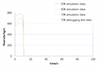 |
Figure 5 Changes in flow rate of faulty pump over time. |
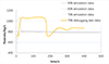 |
Figure 6 Changes in normal operation pump flow rate over time. |
According to Figure 5, it can be seen that under three initial states of 90% FP, 80% FP, and 70% FP of the simulation data, after a feedwater pump trips, the flow rate at the outlet of the faulty pump shows a consistent trend, all of which rapidly decrease to 0 within 2 s. In the debugging test data under the initial load of 70% FP condition, the change in outlet flow rate of the faulty pump is completely consistent with the simulation data, and the flow rate decreases to 0 after about 2 s of pump tripping. The difference lies in the initial operating flow rates are 576 kg/s and 627 kg/s for debugging test data and simulation data, respectively, which reflects a certain difference between the actual operating state of the unit and the ideal state in simulation. Figure 5 shows that the simulation model can accurately predict the flow rate change pattern after the faulty pump trips, based on the time variation data of the faulty pump flow rate.
The key to ensuring the safe and stable operation of the unit and the normal fluctuation of water level in the secondary side of SG without causing reactor shutdown after the main feedwater pump trips is whether the flow rate of the normally operating pump delivered can meet the requirements and whether the heat generated by the reactor can be taken away in a timely manner. According to the simulation data in Figures 6, it can be seen that under the initial power of 90% FP, 80% FP, and 70% FP, when the normal operation pump operates at maximum speed, the pump outlet flow rate is basically the same, reaching to 1052 kg/s. After running at an overspeed for 15 s, the pump’s outlet flow rate decreased to the rated speed and remained stable around 780 kg/s.
The commissioning test data show that the flow rate of the normal operating pump increases rapidly as its speed rises to the maximum speed, with the flow rate corresponding to the maximum speed being 1050 kg/s. After the unit stabilizes, the flow rate provided by the main feedwater pump is approximately 868 kg/s, which has a relatively large error of about 10.1% compared with the simulation data. It should be specifically noted that this discrepancy is not caused by calculation errors; the core reason lies in the fundamental difference in the determination mechanism of the overspeed operation duration of the normal operating pump. In the simulation calculation, to clarify the reference for operating condition analysis and simplify the initial boundary conditions, the overspeed operation duration of the main feedwater pump is set to 15 s (a manually preset fixed value). In contrast, during the commissioning test, the overspeed operation duration is automatically determined and adjusted by the main feedwater speed control system in accordance with the predefined control logic, based on real-time feedback from actual transient conditions (such as steam generator (SG) level deviation and main feedwater flow fluctuation), and the final actual operation duration reaches approximately 140 s. The longer overspeed operation duration enables the feedwater pump to supply more water to the steam generator (SG) during the commissioning test, thereby more fully removing the heat generated by the reactor. This comparison result indicates that the “15-second overspeed operation” boundary condition assumed in the simulation calculation is relatively conservative – it does not incorporate the dynamic adjustment capability of the control system for the overspeed duration. However, such a conservative boundary condition can ensure that the simulation results cover more extreme transient scenarios in safety analysis, which meets the core requirement of “maintaining a reasonable safety margin” for the safety analysis of nuclear power units.
4 Conclusion
A mathematical model for the deaerator, main feedwater pump, and their connected systems was created in this article based on the system and equipment data of a certain HPR1000 nuclear power unit. Through conducting transient simulation calculations of the main feedwater pump tripping, and comparing the simulation data with debugging test data, the following conclusions are drawn:
(1) The unit operates under three initial conditions of 90% FP, 80% FP, and 70% FP was simulated. After one main feedwater pump trips, the speed of normal operation pump reaches to maximum speed, which can effectively supplement the loss of water on the SG secondary side and cooperate with the reactor to quickly reduce its load to 50% FP, avoiding reactor shutdown caused by low steam generator water level;
(2) Comparative analysis shows that the simulation data during the transient process is in good agreement with the debugging test data. The initial and final values of the deaerator pressure have an error of less than 1.5%, and the variation pattern of the deaerator liquid level is basically consistent. The flow rate error of the faulty pump is about 8.1%, the maximum flow rate error of the normal operation pump is about 2‰, and the flow rate error of the normal operation pump after stabilizing at 50% load is about 10.1% between the simulation data and the debugging test data.
(3) The mathematical model established in this paper can effectively predict the pressure and liquid level of the deaerator under transient conditions of single feedwater pump failure and pump tripping, as well as the trend of changes in feedwater flow rate of normal and faulty pumps. The modeling methods used for the main feedwater pump, deaerator and other systems and equipment, as well as the boundary condition assumptions for calculating operating conditions, can provide reference for the design of subsequent HPR1000 nuclear power units.
The innovations of this study are as follows: ① For the first time, a fully coupled mathematical model of “deaerator-main feedwater pump” was constructed on the APROS platform, directly associating the vapor-liquid two-phase equilibrium of the deaerator (Eqs. (1)–(3)) with the speed-torque dynamics of the main feedwater pump (Eqs. (12)–(14)), making up for the deficiency of “emphasizing macro parameters while neglecting equipment coupling” in existing studies; ② Aiming at the unique configuration of 3×50% electric feedwater pumps in HPR1000 units, the transient sequence of “pump tripping-overspeed-load reduction” under different initial loads (90%FP, 80%FP, 70%FP) was quantified. By comparing the actual overspeed time of 140 s with the simulation assumption of 15 s, the safety analysis idea of “conservative boundary conditions” was proposed, providing a transient simulation method reference for the unique feedwater pump configuration of third-generation nuclear power.
However, this study only verified the accuracy of the established model by relying on debugging data under the initial load of 70% FP, and has not covered the transient responses of more complex extreme operating conditions such as unit start-stop processes and low loads (<50% FP). In such conditions, the vapor–liquid two-phase equilibrium of the deaerator is prone to severe fluctuations, and the flow regulation of the main feedwater pump needs to adapt to load changes in a wider range, which places higher requirements on the model’s dynamic prediction capability. In subsequent work, it is necessary to further expand the initial operating conditions to the full load range of 30% FP~100% FP, and systematically verify the generality and reliability of the model in full-load variable-load transient scenarios by combining debugging data from the actual start-stop phase of the unit. This will lay a foundation for the application of the model in the operation analysis of the unit’s full life cycle.
Funding
This research received no external funding.
Conflicts of interest
The authors have nothing to disclose.
Data availability statement
Data will be made available on request.
Author contribution statement
Conceptualization, Chuntian Lu; Methodology, Jianjun Yang; Investigation, Qiang Zhang; Formal Analysis, Hao Chen; Writing – Original Draft Preparation, Qiang Zhang; Writing – Review & Editing, Jianjun Yang; Supervision, Chuntian Lu and Hao Chen.
References
- G. Pan, Y. Zheng, N. Chen, Numerical calculation of three-dimensional flow field of feed water pump for ultra supercritical units, Thermal Power Generation 41(3), 4 (2012). [Google Scholar]
- H. Li, B. Song, R. Yang, Modeling and simulation analysis of feedwater pump turbine, Steam Turbine Technol. 50(1), 3 (2008). [Google Scholar]
- W. Li, L. Cui, J. Kang, et al., Optimization of the feedwater control system for a 600MW unit based on Matlab/Simulink dynamic modeling. Thermal Power Generation 38(12), 82–87 (2009). [Google Scholar]
- L. Fu, Improvement of water supply control system for 2×142MW heating unit. China Electric Power (5), 81–84 (2005). [Google Scholar]
- D. Li, F. Sun, Z. Jiao, Simulation modeling and implementation of feedwater pumps considering cavitation effects. Comput. Simul. 2005 (2), 67–69 (2005). [Google Scholar]
- X. Cheng, P. Yan, Y. Fu, et al., Transient analysis of a single feedwater pump tripping during rated power operation of an AP1000 nuclear power plant. China Electric Power (8), (2015). [Google Scholar]
- B. Zeng, X. Shang, X. Huang, Transient impact analysis and improvement of the main feedwater pump of M310 nuclear power plant. Elect. Technol. (16), 3 (2021). [Google Scholar]
- Y. Hu, Input selection and margin value analysis of the main feedwater pump design for pressurized water reactor nuclear power plants. Nucl. Sci. Eng. (S1), 5 (2010). [Google Scholar]
- L. Zhao, Modeling and simulation of the secondary circuit of Hongyanhe nuclear power units based on Apollo (Shanghai Electric Power University, 2024). [Google Scholar]
- A. Sun, M. Li, S. Yang, et al., Accident simulation and control strategy of feedwater system of sodium-cooled fast reactor. Prog. Nuclear Energy 172, 105214 (2024). [Google Scholar]
- Y. Park, S. Jeon, et al., Effect of passive auxiliary feedwater system on mitigation of DEC accidents: Part I. MSGTR, SBLOCA-LOSI, and SBO. Ann. Nucl. Energy 206, 110643 (2024). [Google Scholar]
- W. Yin, Research on dynamic modeling and control methods of marine condensing systems (Harbin Engineering University, 2008). [Google Scholar]
- J. Wu, Z. Xu, X. Ma, Simulation study on water level control model of deaerator in nuclear power plants. Thermal Power Generation (3), 5 (2014). [Google Scholar]
- P. Sun, X. Zhang, et al., Modeling and simulation of feedwater control system with multiple once-through steam generators in a sodium-cooled fast reactor (II): Control system simulation. Ann. Nucl. Energy 149, 107780 (2020). [Google Scholar]
- K. Deng, C. Yang, H. Chen, et al., Start-Up and dynamic processes simulation of supercritical once-through boiler. Appl. Therm. Eng. 115, 937–946 (2017). [Google Scholar]
- T.N. Nguyen, R. Ponciroli, T. Kibler, et al., A physics-based parametric regression approach for feedwater pump system diagnosis. Ann. Nucl. Energy 166, 108692 (2022). [Google Scholar]
Cite this article as: Yang J, Lu C, Zhang Q & Chen H. Trip transient analysis on the main feedwater pump of HPR1000, Res. Des. Nucl. Eng. 2, 2025008 (2026). https://doi.org/10.1051/rdne/2025008.
All Figures
|
Figure 1 Thermal system diagram of the secondary loop. |
| In the text | |
|
Figure 2 Schematic diagram of deaerator water level calculation. |
| In the text | |
|
Figure 3 Pressure variation of deaerator over time. |
| In the text | |
|
Figure 4 Changes in deaerator water level over time. |
| In the text | |
|
Figure 5 Changes in flow rate of faulty pump over time. |
| In the text | |
|
Figure 6 Changes in normal operation pump flow rate over time. |
| In the text | |
Current usage metrics show cumulative count of Article Views (full-text article views including HTML views, PDF and ePub downloads, according to the available data) and Abstracts Views on Vision4Press platform.
Data correspond to usage on the plateform after 2015. The current usage metrics is available 48-96 hours after online publication and is updated daily on week days.
Initial download of the metrics may take a while.