Application of multi-GPU parallel finite element software (GFE) in seismic analysis of nuclear power structures

Shengtao Cao; Zhidong Gao; Mi Zhao; Yangzhou Wu; Zhishan Li; Xiuli Du

doi:10.1051/rdne/2025002

All issues

Volume 1 (2025)

Res. Des. Nucl. Eng., 1 (2025) 2025002

Full HTML

Open Access

Issue		Res. Des. Nucl. Eng. Volume 1, 2025


Article Number		2025002
Number of page(s)		7
DOI		https://doi.org/10.1051/rdne/2025002
Published online		04 July 2025

Research & Design of Nuclear Engineering, 1, 2025002 (2025)

Research Article

Application of multi-GPU parallel finite element software (GFE) in seismic analysis of nuclear power structures

Shengtao Cao¹, Zhidong Gao², Mi Zhao²^*, Yangzhou Wu², Zhishan Li¹ and Xiuli Du²

¹ Research Institute of Tsinghua, Pearl River Delta, Guangzhou 510530, Guangdong, China
² Key Laboratory of Urban Security and Disaster Engineering of Ministry of Education, Beijing University of Technology, Beijing 100124, China

^* Corresponding author: zhaomi@bjut.edu.cn

Received: 14 February 2025
Accepted: 17 April 2025

Abstract

The safety of nuclear power structure is very important. The establishment of a refined fine finite element model is beneficial to the dynamic analysis of nuclear power structure, but it brings challenges to the computational efficiency. In this paper, a self-developed finite element software based on multi-GPU parallel explicit algorithm (GFE) is firstly introduced. Using the GFE software, dynamic response of nuclear power structures considering soil-structure interaction (SSI) under seismic load is analyzed and compared with the commercial software. The calculation results show that the results obtained from the GFE software is consistent with that obtained from the commercial software. Compared with the general commercial software, the GFE software has higher computational efficiency. The calculation time of GFE software for the seismic analysis is respectively about 1/7 that of the general commercial software.

Key words: Nuclear power structures / GFE software, seismic analysis / Soil-structure interaction

© The Author(s) 2025. Published by EDP Sciences and China Science Publishing & Media Ltd.

This is an Open Access article distributed under the terms of the Creative Commons Attribution License (https://creativecommons.org/licenses/by/4.0), which permits unrestricted use, distribution, and reproduction in any medium, provided the original work is properly cited.

1 Introduction

In the current global resource constraints, nuclear power, as a clean and efficient resource, is receiving increasing national attention [1]. The safety first has remained an important foundation for the sustainable development of nuclear power plants [2, 3]. In 2001, the terrorist attack on the World Trade Centre in New York City impacted by a large commercial aircraft occurred in the USA. And in 2011, the 9.0 magnitude earthquake which occurred in Fukushima, Japan, severely damaged the nuclear power plant and the surrounding infrastructure [4]. After the 9.11 incident and the Fukushima nuclear accident, the safety requirements of nuclear power plants have been increasingly raised. Currently, the problems of resistance to large aircraft impacts and rare earthquakes together with the secondary disasters, are the main issues threatening the structural safety of nuclear power plants.

In recent years, many scholars have studied the seismic response of nuclear power structure [5–12]. Suitable bedrock sites for the nuclear power plants are becoming rare, and more and more nuclear power plants are being built on non-bedrock sites [12, 13]. The soil-structure interaction (SSI) effects on the seismic response of the nuclear power plants need to be considered in this case [14–17]. The direct finite element method can accurately simulate the SSI effects. Direct models are used by most scholars to investigate the SSI effects on the seismic response of nuclear power plants [12, 13]. The artificial boundary needs to be implemented at the truncated boundary of the soil domain in order to consider the effect of radiation damping. Moreover, site responses need to be performed and equivalent seismic loads need to be applied at truncated artificial boundaries [18–21]. The above process is not convenient to realize in the current commercial finite element software. For example, Zhao et al. [22] used FORTRAN to produce an assistant program for inputting equivalent nodal loads and setting viscoelastic boundaries. The calculation results were combined into the INP file to achieve the setting of artificial boundary conditions in the finite element model. The pre and post-processing operations are very complicated when using the existing finite element software for SSI analysis, and the computational efficiency of the SSI system model is not efficient.

In order to improve the computational efficiency for investigating the seismic problem of nuclear power structures, a self-developed finite element software based on multi-GPU parallel explicit algorithm (GFE) is used in this paper. The details of the GFE software are described in Section 2. In Section 3, the seismic response of nuclear power structures considering SSI is investigated using the GFE software. The conclusion is given in Section 4.

2 GFE software

The finite element method based on CPU may not always provide the necessary computational efficiency for scientific research and practical engineering, especially when dealing with nonlinear dynamic problems. Recent years have seen a considerable increase in the speed of arithmetic processing. The utilisation of GPU parallel acceleration technology has emerged as a highly effective strategy to enhance computational efficiency. However, contemporary general-purpose finite element analysis software predominantly employs implicit algorithms for GPU parallelism. The GFE software is a high-performance finite element software developed based on multi-GPU parallel computing architecture. GFE can realise the parallelism of nonlinear dynamical explicit calculations on multiple GPUs. The GFE software contains three modules: pre-processing, solver and post-processing. The GFE software can use multi-GPU for large-scale parallel computation, which has significant advantages in terms of model refinement, solving speed, and solving scale [23]. As shown in Figure 1, based on multi-GPU parallel architecture, the GFE software achieves fine-grained parallel computation for finite element explicit dynamics analysis, which significantly improves the computational efficiency. Therefore, the seismic response of the nuclear power plant considering the SSI effects can be computed efficiently using the GFE.

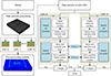Fig. 1

Multi-GPU parallel computing for GFE explicit dynamics analysis.

It should be pointed out that the GFE software also integrates the necessary tools for seismic SSI analysis, such as viscoelastic boundary, site response and seismic input, etc. It also develops many elastic-plastic constitutive models of soil and concrete, which can be easily used for seismic and impact analysis of nuclear power structures.

3 Seismic analysis of nuclear power structure considering SSI

3.1 Nuclear structure and earthquake

The nuclear power plant consists of three parts, including an auxiliary plant, a concrete foundation slab, and a containment plant, as shown in Figure 2. The total structural height of the containment plant is 73 m, with an underground section of 10.46 m. The radius of the containment plant is 21.5 m and the wall thickness is 1.5 m. The concrete of the containment plant is C60 with Young’s modulus of 3.60 × 1010 N/m², density of 2500 kg/m³ and Poisson’s ratio of 0.20. The concrete of the auxiliary plant and foundation slab is C40 with Young’s modulus of 3.25 × 1010 N/m², density of 2500 kg/m³ and Poisson’s ratio of 0.20. A fine finite element model of the nuclear power plant was developed using the GFE, as shown in Figure 3. The concrete foundation slab was modelled using solid element with a grid size of 1.0 m, and the nuclear power plant was modelled using shell element with a grid size of 0.5 m.

Fig. 2

Geometrical model of nuclear structure.

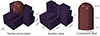Fig. 3

Finite element models of nuclear structure.

The Kobe earthquake is used in this paper with the peak acceleration adjusted to 0.15 g. The acceleration time-history curves and Fourier amplitude spectra of Kobe earthquake is presented in Figure 4.

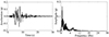Fig. 4

Acceleration time-history curves and Fourier amplitude spectra of the Kobe earthquake.

3.2 Earthquake input method based on viscous spring artificial boundary

The finite element model of the SSI system is given in Figure 5. The length, width and height of the soil model are 500 m, 400 m and 70 m, respectively. The soil is modelled using solid elements. The mesh size of the soil is 4 m, which meets the requirement that the minimum wavelength is less than 1/8 to 1/10 [24]. The shear wave velocity of the soil was 2400 m/s, with Young’s modulus of 40.07 × 1010 N/m², density of 2400 kg/m³ and Poisson’s ratio of 0.20. The viscous spring artificial boundary is used on the SSI model boundaries to simulate the radiation damping effect in the infinite domain.

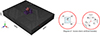Fig. 5

Finite element modeling of soil-structure systems.

The motion equations for the SSI system can be written as

$[\begin{matrix} M_{RR} & M_{RB} \\ M_{BR} & M_{BB} \end{matrix}] {\begin{matrix} ü_{R} \\ ü_{B} \end{matrix}} + [\begin{matrix} C_{RR} & C_{RB} \\ C_{BR} & C_{BB} \end{matrix}] {\begin{matrix} {\dot{u}}_{R} \\ {\dot{u}}_{B} \end{matrix}} + [\begin{matrix} K_{RR} & K_{RB} \\ K_{BR} & K_{BB} \end{matrix}] {\begin{matrix} u_{R} \\ u_{B} \end{matrix}} = {\begin{matrix} 0 \\ f_{B} \end{matrix}},$ $\left[\begin{array}{cc}{\mathbf{M}}_{{RR}}& {\mathbf{M}}_{{RB}}\\ {\mathbf{M}}_{{BR}}& {\mathbf{M}}_{{BB}}\end{array}\right]\left\{\enspace \begin{array}{c}{\mathbf{\mathbf{Error:000FC} }}_R\\ {\mathbf{\mathbf{Error:000FC} }}_B\end{array}\right\}+\left[\begin{array}{cc}{\mathbf{C}}_{{RR}}& {\mathbf{C}}_{{RB}}\\ {\mathbf{C}}_{{BR}}& {\mathbf{C}}_{{BB}}\end{array}\right]\left\{\begin{array}{c}{\stackrel{\dot }{\mathbf{u}}}_R\\ {\stackrel{\dot }{\mathbf{u}}}_B\end{array}\right\}+\left[\begin{array}{cc}{\mathbf{K}}_{{RR}}& {\mathbf{K}}_{{RB}}\\ {\mathbf{K}}_{{BR}}& {\mathbf{K}}_{{BB}}\end{array}\right]\left\{\begin{array}{c}{\mathbf{u}}_R\\ {\mathbf{u}}_B\end{array}\right\}=\left\{\begin{array}{c}\mathbf{0}\\ {\mathbf{f}}_B\end{array}\right\},$ (1)

where the subscripts B and R denote the degrees of freedom of the artificial boundary and the rest of the finite domain, respectively; u, ü, and $\dot{u}$ $\stackrel{\dot }{\mathbf{u}}$ represent absolute displacement, velocity, and acceleration, respectively; K, C and M denote the stiffness, damping, and mass matrices of the SSI system, respectively; and f_B is the action force vector provided by the infinite domain.

The total reaction at the artificial boundary is divided into the scattered field and the free field:

$f_{B} = f_{B}^{S} + f_{B}^{F},$ ${\mathbf{f}}_B={\mathbf{f}}_B^S+{\mathbf{f}}_B^F,$ (2)

$u_{B} = u_{B}^{S} + u_{B}^{F},$ ${\mathbf{u}}_B={\mathbf{u}}_B^S+{\mathbf{u}}_B^F,$ (3)

${\dot{u}}_{B} = {\dot{u}}_{B}^{S} + {\dot{u}}_{B}^{F},$ ${\stackrel{\dot }{\mathbf{u}}}_B={\stackrel{\dot }{\mathbf{u}}}_B^S+{\stackrel{\dot }{\mathbf{u}}}_B^F,$ (4)

where the free field is denoted by the superscript F, which is determined by the site response analysis, and the scattered field is denoted by the superscript S.

Using the viscous spring artificial boundary condition to simulate the scattered field, and the force and motion relationship of the scattered field can be written as

$f_{B}^{S} = - K_{B}^{\infty} u_{B}^{S} - C_{B}^{\infty} {\dot{u}}_{B}^{S},$ ${\mathbf{f}}_B^S=-{\mathbf{K}}_B^{\infty }{\mathbf{u}}_B^S-{\mathbf{C}}_B^{\infty }{\stackrel{\dot }{\mathbf{u}}}_B^S,$ (5)

_where $K_{B}^{\infty} = [\begin{matrix} K_{N} & 0 & 0 \\ 0 & K_{T} & 0 \\ 0 & 0 & K_{T} \end{matrix}]$ ${\mathbf{K}}_B^{\infty }=\left[\begin{array}{ccc}{K}_N& 0& 0\\ 0& {K}_T& 0\\ 0& 0& {K}_T\end{array}\right]$ _and $C_{B}^{\infty} = [\begin{matrix} C_{N} & 0 & 0 \\ 0 & C_{T} & 0 \\ 0 & 0 & C_{T} \end{matrix}]$ ${\mathbf{C}}_B^{\infty }=\left[\begin{array}{ccc}{C}_N& 0& 0\\ 0& {C}_T& 0\\ 0& 0& {C}_T\end{array}\right]$ _{are the stiffness and damping matrices, respectively. The subscript N and T denote the normal and tangential directions of the boundary, respectively. The stiffness and damping matrix consist of spring and damping coefficients at the viscous spring artificial boundary.}

Substituting, the Eqs. (3) and (4) into Eq. (5), then into Eq. (2), and finally into Eq. (1), the finite element equation is obtained after collation as

$[\begin{matrix} M_{RR} & M_{RB} \\ M_{BR} & M_{BB} \end{matrix}] {\begin{matrix} ü_{R} \\ ü_{B} \end{matrix}} + [\begin{matrix} C_{RR} & C_{RB} \\ C_{BR} & C_{BB} + C_{B}^{\infty} \end{matrix}] {\begin{matrix} {\dot{u}}_{R} \\ {\dot{u}}_{B} \end{matrix}} + [\begin{matrix} K_{RR} & K_{RB} \\ K_{BR} & K_{BB} + K_{B}^{\infty} \end{matrix}] {\begin{matrix} u_{R} \\ u_{B} \end{matrix}} = {\begin{matrix} 0 \\ f_{B}^{F} + K_{B}^{\infty} u_{B}^{F} + C_{B}^{\infty} {\dot{u}}_{B}^{F} \end{matrix}} .$ $\left[\begin{array}{cc}{\mathbf{M}}_{{RR}}& {\mathbf{M}}_{{RB}}\\ {\mathbf{M}}_{{BR}}& {\mathbf{M}}_{{BB}}\end{array}\right]\left\{\begin{array}{c}{\mathbf{\mathbf{Error:000FC} }}_R\\ {\mathbf{\mathbf{Error:000FC} }}_B\end{array}\right\}+\left[\begin{array}{cc}{\mathbf{C}}_{{RR}}& {\mathbf{C}}_{{RB}}\\ {\mathbf{C}}_{{BR}}& {\mathbf{C}}_{{BB}}+{\mathbf{C}}_B^{\infty }\end{array}\right]\left\{\begin{array}{c}{\stackrel{\dot }{{u}}}_R\\ {\stackrel{\dot }{{u}}}_B\end{array}\right\}+\left[\begin{array}{cc}{\mathbf{K}}_{\mathrm{RR}}& {\mathbf{K}}_{\mathrm{RB}}\\ {\mathbf{K}}_{\mathrm{BR}}& {\mathbf{K}}_{\mathrm{BB}}+{\mathbf{K}}_B^{\infty }\end{array}\right]\left\{\begin{array}{c}{\mathbf{u}}_R\\ {\mathbf{u}}_B\end{array}\right\}=\left\{\begin{array}{c}0\\ {\mathbf{f}}_B^F+{\mathbf{K}}_B^{\infty }{\mathbf{u}}_B^F+{\mathbf{C}}_B^{\infty }{\stackrel{\dot }{\mathbf{u}}}_B^F\end{array}\right\}.$ (6)

3.3 Results

Three reference points are selected in the SSI system as point A, point B and point C. The three reference points are located on the soil domain, on the ancillary plant and on the containment plant, respectively. Moreover, other three points are also selected at the top, central and bottom of the containment plant namely C1, C2 and C3. Schematic of reference points for the SSI system and containment plant is given in Figure 6. In addition, the peak floor acceleration, the peak relative floor displacement, and the floor response spectra of the containment under seismic loading are presented.

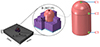Fig. 6

Schematic of reference points for the SSI system.

The acceleration time-history curves and displacement time-history curves of point A, point B and point C are given in Figure 7. The peak floor acceleration, the peak relative floor displacement, and the floor response spectra of the containment plant are given in Figure 8. The seismic responses of the containment plant are obtained by GFE and ABAQUS software, respectively. The time-history curves of the reference points obtained by GFE and ABAQUS are essentially coincident. The peak floor acceleration of the containment plant obtained by GFE and ABAQUS is 4.05 m/s² and 3.97 m/s², respectively. The peak relative floor displacement of the containment plant obtained by GFE and ABAQUS is 5.01 mm and 4.93 mm, respectively. The peak value of the floor response spectra of the containment plant obtained by GFE and ABAQUS is 25.58 m/s² and 25.88 m/s², respectively. The seismic response of the containment plant, including peak floor acceleration, peak relative floor displacement and the floor response spectra, obtained from GFE and ABAQUS, had errors of 1.97%, 1.59% and 1.14%, respectively. The results are the same for the two software ABAQUS and GFE.

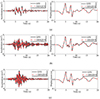Fig. 7

The curves of the acceleration time-history and displacement time-history. (a) Results at point A; (b) Results at point B; (c) Results at point C.

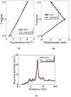Fig. 8

Seismic response of containment under Kobe earthquakes. (a) Peak floor acceleration (b) Peak relative floor displacement; (c) Floor response spectra at Point C1.

The total number of degrees of freedom of the SSI system is 887667 and the total number of elements is 231399. The seismic response of the SSI system was calculated using ABAQUS software spending 125 min. The computer was configured with a 12-core CPU. The seismic response of the SSI system was calculated using GFE software spending 19 min. The computer was configured with a 2080 dual-card GPU. With the same computer configuration, the calculation time using GFE is about one-seventh of ABAQUS, and the calculation efficiency is significantly improved.

4 Conclusion

In this paper, the GFE finite element software based on multi-GPU parallel explicit algorithm is firstly introduced. A refined finite element model of a nuclear power structure is established using the GFE. The seismic response of the nuclear power structure considering soil-structure interaction is investigated. The results obtained by commercial software are used as a reference. The results obtained from the GFE software is consistent with that obtained from the commercial software, and the computational efficiency has been improved.

Funding

This work presented in this paper is supported by National Natural Science Foundation of China (52338001).

Conflicts of interest

The authors declare no conflict of interest.

Data availability statement

Data will be made available on request.

Author contribution statement

All the researchers worked equally. Each of them helped in the writing of this paper.

References

World Nuclear Association, World nuclear performance report (2023). [Google Scholar]
China Earthquake Administration (CEA), Standard for seismic design of nuclear power plants, GB 50267–2019 (China Planning Press, Beijing, 2019). [Google Scholar]
American Society of Civil Engineers (ASCE), Seismic analysis of safety-related nuclear structures and commentary (ASCE/SEI Standard, Reston, VA, 2017). [Google Scholar]
Y. Shumuta, Damage and Restoration of Electric Power System due to the 2011 Earthquake off the Pacific Coast of Tōhoku-Effects of a Damage Estimation System for Electric Power Distribution Equipment (RAMPEr) (International Efforts in Lifeline Earthquake Engineering. ASCE, 2014), pp. 81–88. [Google Scholar]
R.Y. Mei, J.B. Li, G. Lin, et al., Evaluation of the vibration response of third generation nuclear power plants with isolation technology under large commercial aircraft impact. Prog. Nucl. Energy 120, 103230 (2020). [Google Scholar]
Y. Liu, J.B. Li, G. Lin, Seismic performance of advanced three-dimensional base-isolated nuclear structures in complex-layered sites, Eng. Struct. 289, 116247 (2023). [Google Scholar]
Z. Zhou, J. Wong, S. Mahin, Potentiality of using vertical and three-dimensional isolation systems in nuclear structures, Nucl. Eng. Technol. 48, 1237–1251 (2016). [Google Scholar]
M. Forni, A. Poggianti, Dusi A. Seismic isolation of nuclear power plants, in: World Conference on Earthquake Engineering (2012), pp. 636–639. [Google Scholar]
R.S. Malushte, S.A. Whittaker, Survey of past base isolation applications in nuclear power plants and challenges to industry/regulatory acceptance, in: Transactions of the 18th International Conference on Structural Mechanics in Reactor Technology (2005), pp. 3404–3410. [Google Scholar]
Y.Z. Wu, D. Yao, L.H. Wu, et al., Seismic performance investigation of PCS water tank designed as tuned mass damper (TMD) for nuclear containment plant considering soil-structure interaction, Soil Dyn. Earthq. Eng. 186, 108937 (2024). [Google Scholar]
Z.Q. Sun, M. Zhao, Z.D. Gao, et al., Seismic mitigation performance of a periodic foundation for nuclear power structures considering soil-structure interactions, Soil Dyn. Earthq. Eng. 184, 108814 (2024). [Google Scholar]
J.P. Wolf, Dynamic soil-structure interaction (Prentice Hall, Englewood Cliffs, NJ, 1985). [Google Scholar]
J.P. Wolf, Dynamic soil-structure interaction analysis in time-domain (Prentice-Hall, Englewood Cliffs, NJ, 1988). [Google Scholar]
L. Tunon-Sanjur, R.S. Orr, S. Tinic, D.P. Ruiz, Finite element modeling of the AP1000 nuclear island for seismic analyses at generic soil and rock sites, Nucl Eng Des. 237, 147–185 (2007). [Google Scholar]
H.K. Mistry, D. Lombardi, Role of SSI on seismic performance of nuclear reactors: a case study for a UK nuclear site, Nucl. Eng. Des. 364, 110691 (2020). [Google Scholar]
J.B. Li, M. Chen, Z. Li, Improved soil-structure interaction model considering time-lag effect, Comput. Geotech. 148, 104835 (2022). [Google Scholar]
H. Lv, S.L. Chen, Seismic response characteristics of nuclear island structure at generic soil and rock sites, Earthq. Eng. Eng. Vib. 22, 667–688 (2023). [Google Scholar]
J.B. Liu, Y.X. Du, Z.Y. Wang, et al., 3D viscous-spring artificial boundary in time domain, Earthq. Eng. Eng. Vib. 1(5), 93–101 (2006). [Google Scholar]
X.L. Du, M. Zhao, J.T. Wang, A stress artificial boundary in FEA for near-field wave problem, Chin. J. Theor. Appl. Mech. 38 (1), 49–56 (2006), in Chinese. [Google Scholar]
P.P. Martin, H.B. Seed, A computer program for the non-linear analysis of vertically propagating shear waves in horizontally layered deposits (University of California at Berkeley, San Francisco, 1978). [Google Scholar]
A. Amorosi, D. Boldini, Numerical modelling of the transverse dynamic behavior of circular tunnels in clayey soils, Soil Dyn. Earthq. Eng. 29, 1059–1072 (2009). [Google Scholar]
M. Zhao, H. Yin, X. Du, et al., 1D finite element artificial boundary method for layered half space site response from obliquely incident earthquake, Earthq. Struct. 22, 173–194 (2015). [Google Scholar]
M. Zhao, Q. Ding, S. Cao, et al., Large-scale seismic soil-structure interaction analysis via efficient finite element modeling and multi-GPU parallel explicit algorithm. Comput. Aided Civ. Infrastruct. Eng. 39, 1886–1908 (2024). [Google Scholar]
G.B. Warburton, Optimum absorber parameters for various combinations of response and excitation parameters, Earthq. Eng. Struct. Dyn. 10, 381–401 (1982). [Google Scholar]

Cite this article as: Cao S, Gao Z, Zhao M, Wu Y, Li Z, et al. Application of multi-GPU parallel finite element software (GFE) in seismic analysis of nuclear power structures, Res. Des. Nucl. Eng. 1, 2025002 (2025), https://doi.org/10.1051/rdne/2025002.

All Figures

	Fig. 1 Multi-GPU parallel computing for GFE explicit dynamics analysis.
In the text

	Fig. 2 Geometrical model of nuclear structure.
In the text

	Fig. 3 Finite element models of nuclear structure.
In the text

	Fig. 4 Acceleration time-history curves and Fourier amplitude spectra of the Kobe earthquake.
In the text

	Fig. 5 Finite element modeling of soil-structure systems.
In the text

	Fig. 6 Schematic of reference points for the SSI system.
In the text

	Fig. 7 The curves of the acceleration time-history and displacement time-history. (a) Results at point A; (b) Results at point B; (c) Results at point C.
In the text

	Fig. 8 Seismic response of containment under Kobe earthquakes. (a) Peak floor acceleration (b) Peak relative floor displacement; (c) Floor response spectra at Point C1.
In the text

Current usage metrics show cumulative count of Article Views (full-text article views including HTML views, PDF and ePub downloads, according to the available data) and Abstracts Views on Vision4Press platform.

Data correspond to usage on the plateform after 2015. The current usage metrics is available 48-96 hours after online publication and is updated daily on week days.

Initial download of the metrics may take a while.